Our goal is to develop a framework to measure the quality of gate implementations on quantum computers.
The general strategy is to create random circuits and let them run on the hardware. By comparing the final and initial states, we can detect errors and assign a score to the quantum hardware based on the fidelity between the final and initial states.
A stabilizer state is a state \(|\psi\rangle\) for which there exists a subgroup \(S \subseteq \mathcal{P}_n\) of the Pauli group on \(n\) qubits such that
$$ s\,|\psi\rangle = |\psi\rangle \quad \forall\, s \in S. $$In the language of PauliSum, a stabilizer state is described by:
The phases of the stabilizer generators uniquely identify the stabilized state.
We model noise using the Kraus operator formalism. Assume that at the initial time the quantum state is pure and separable between the system (\(s\)) and the environment (\(e\)):
$$ \rho_0 = \rho^s_0 \otimes |e_0\rangle\langle e_0|, $$where \(|e_0\rangle\) is a generally unknown environmental state. Since the composite system is closed, the joint state evolves unitarily:
$$ \rho_{\mathrm{out}} = U_{se}\left(\rho^s_0 \otimes |e_0\rangle\langle e_0|\right) U_{se}^\dagger. $$Tracing out the environment yields the reduced dynamics of the system:
$$ \rho^s_{\mathrm{out}} = \mathrm{Tr}_e\!\Big[U_{se}\left(\rho^s_0 \otimes |e_0\rangle\langle e_0|\right) U_{se}^\dagger\Big] = \sum_i \langle e_i | U_{se} | e_0 \rangle\;\rho^s_0\;\langle e_0 | U_{se}^\dagger | e_i \rangle. $$Defining the Kraus operators \(K_i U_s = \langle e_i | U_{se} | e_0 \rangle\), the map takes the standard Kraus form:
$$ \rho^s_{\mathrm{out}} = \sum_i K_i\,U_s \,\rho_0^s\,U_s^\dagger \, K_i^\dagger, \label{eq:kraus} \tag{1} $$with the completeness (trace-preservation) relation
$$ \sum_i K_i^\dagger K_i = \mathbb{1}. $$We consider an error model consisting of an ideal application of each quantum gate followed by noise acting on each of the qubits involved. While our protocols work with arbitrary (Clifford) noise, we focus on dephasing and depolarizing channels. For single-qubit unitaries \(U\) (with \(m=1\)), the Kraus operators are:
Dephasing:
$$ K_0 = \sqrt{p_0}\,\mathbb{1}, \qquad K_1 = \sqrt{1 - p_0}\,Z, \tag{2a} $$Depolarizing:
$$ K_0 = \sqrt{p_0}\,\mathbb{1}, \qquad K_i = \sqrt{\frac{1 - p_0}{3}}\,\sigma_i, \quad i = 1,2,3, \tag{2b} $$where \(\sigma_i\) denotes the Pauli operator \(X\), \(Y\), or \(Z\) for \(i=1,2,3\) respectively, and \(p_0\) is the probability of no error occurring. For \(m \geq 2\) qubits, the corresponding channels are constructed by taking all tensor products of the possible permutations of \(m\) operators \(K_i\) (one per qubit). For these models, we use uncorrelated noise between qubits.
In practice, we convert the Kraus operators to their corresponding (Clifford) gates and apply these “noise gates” to the state obtained after applying the ideal gate. We thus work consistently in the gate-based quantum computation model. The initial stabilizer state is then mapped to a (different) stabilizer state by the noisy Clifford circuit.
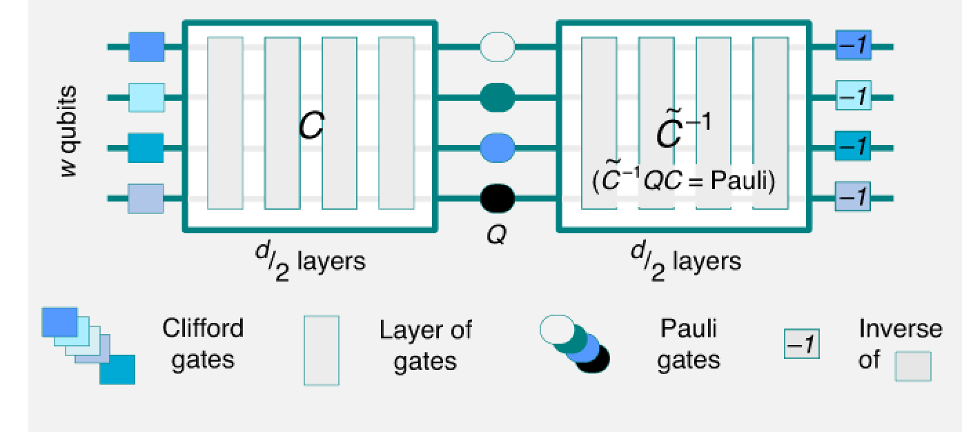
The idea is to build Clifford circuits that, by construction, in the absence of noise return the initial state. The effect of noise is then to deviate the final state from the expected one (the initial state). By measuring the fidelity between the noisy final state and the initial state, we can assign a score to each circuit.
Given the Clifford nature of the circuit, we can work in symplectic space. The obvious advantage is that we do not deal with exponentially large Hilbert spaces. The challenge is that we do not want to evaluate the summation in Eq. \(\eqref{eq:kraus}\) directly. We therefore use a ballistic approach: rather than following the full unitary evolution of the system, we apply quantum jumps whenever noise is applied. Each Kraus operator has an associated probability, by which we randomly select one. The system therefore undergoes a ballistic evolution where only one of the possible “noise paths” is followed. In a sense, we are “measuring” the system with noise after each gate application. This approach is very similar to [1].
To verify that this approach works, we can calculate the Ballistic Accuracy (BA). We use the fidelity defined as
$$ F(\rho, \sigma) = \left(\mathrm{Tr}\sqrt{\sqrt{\rho}\,\sigma\,\sqrt{\rho}}\right)^2. \label{eq:fidelity} \tag{4} $$BA measures the agreement between the average state obtained via the ballistic symplectic evolution over several stochastic runs and the state obtained from the exact unitary evolution (as opposed to the fidelity between noisy and ideal states used for benchmarking). In general, to compute BA accurately, we need to run an exponential number of experiments.
The goal is that, once we establish that the ballistic approach accurately reproduces the unitary evolution, we can run it on the circuits we want to test only a number of times necessary to collect enough statistics (i.e., to reduce the variance below a certain threshold).
We then proceed as follows: